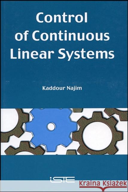
Control of Continuous Linear Systems » książka


Control of Continuous Linear Systems
ISBN-13: 9781905209125 / Angielski / Twarda / 2006 / 350 str.
Control of Continuous Linear Systems
ISBN-13: 9781905209125 / Angielski / Twarda / 2006 / 350 str.
(netto: 804,52 VAT: 5%)
Najniższa cena z 30 dni: 811,02 zł
ok. 22 dni roboczych.
Darmowa dostawa!
This book contains more than 150 problems and solutions on the control of linear continuous systems. The main definitions and theoretical tools are summarized at the beginning of each chapter, after which the reader is guided through the problems and how to solve them. The author provides coverage of the ideas behind the developments of the main PID tuning techniques, as well as presenting the proof of the Routh-Hurwitz stability criterion and giving some new results dealing with the design of root locus.
Wydanie ilustrowane
Introduction xiii
Chapter 1. Introduction to Signals and Systems 1
Yannick BERTHOUMIEU, Eric GRIVEL and Mohamed NAJIM
1.1. Introduction 1
1.2. Signals: categories, representations and characterizations 1
1.2.1. Definition of continuous–time and discrete–time signals 1
1.2.2. Deterministic and random signals 6
1.2.3. Periodic signals 8
1.2.4. Mean, energy and power 9
1.2.5. Autocorrelation function 12
1.3. Systems 15
1.4. Properties of discrete–time systems 16
1.4.1. Invariant linear systems 16
1.4.2. Impulse responses and convolution products 16
1.4.3. Causality 17
1.4.4. Interconnections of discrete–time systems 18
1.5. Bibliography 19
Chapter 2. Discrete System Analysis 21
Mohamed NAJIM and Eric GRIVEL
2.1. Introduction 21
2.2. The z–transform 21
2.2.1. Representations and summaries 21
2.2.2. Properties of the z–transform 28
2.2.2.1. Linearity 28
2.2.2.2. Advanced and delayed operators 29
2.2.2.3. Convolution 30
2.2.2.4. Changing the z–scale 31
2.2.2.5. Contrasted signal development 31
2.2.2.6. Derivation of the z–transform 31
2.2.2.7. The sum theorem 32
2.2.2.8. The final–value theorem 32
2.2.2.9. Complex conjugation 32
2.2.2.10. Parseval s theorem 33
2.2.3. Table of standard transform 33
2.3. The inverse z–transform 34
2.3.1. Introduction 34
2.3.2. Methods of determining inverse z–transforms 35
2.3.2.1. Cauchy s theorem: a case of complex variables 35
2.3.2.2. Development in rational fractions 37
2.3.2.3. Development by algebraic division of polynomials 38
2.4. Transfer functions and difference equations 39
2.4.1. The transfer function of a continuous system 39
2.4.2. Transfer functions of discrete systems 41
2.5. Z–transforms of the autocorrelation and intercorrelation functions 44
2.6. Stability 45
2.6.1. Bounded input, bounded output (BIBO) stability 46
2.6.2. Regions of convergence 46
2.6.2.1. Routh s criterion 48
2.6.2.2. Jury s criterion 49
Chapter 3. Frequential Characterization of Signals and Filters 51
Eric GRIVEL and Yannick BERTHOUMIEU
3.1. Introduction 51
3.2. The Fourier transform of continuous signals 51
3.2.1. Summary of the Fourier series decomposition of continuous signals 51
3.2.1.1. Decomposition of finite energy signals using an orthonormal base 51
3.2.1.2. Fourier series development of periodic signals 52
3.2.2. Fourier transforms and continuous signals 57
3.2.2.1. Representations 57
3.2.2.2. Properties 58
3.2.2.3. The duality theorem 59
3.2.2.4. The quick method of calculating the Fourier transform 59
3.2.2.5. The Wiener–Khintchine theorem 63
3.2.2.6. The Fourier transform of a Dirac comb 63
3.2.2.7. Another method of calculating the Fourier series development of a periodic signal 66
3.2.2.8. The Fourier series development and the Fourier transform 68
3.2.2.9. Applying the Fourier transform: Shannon s sampling theorem 75
3.3. The discrete Fourier transform (DFT) 78
3.3.1. Expressing the Fourier transform of a discrete sequence 78
3.3.2. Relations between the Laplace and Fourier z–transforms 80
3.3.3. The inverse Fourier transform 81
3.3.4. The discrete Fourier transform 82
3.4. The fast Fourier transform (FFT) 86
3.5. The fast Fourier transform for a time/frequency/energy representation of a non–stationary signal 90
3.6. Frequential characterization of a continuous–time system 91
3.6.1. First and second order filters 91
3.6.1.1. 1st order system 91
3.6.1.2. 2nd order system 93
3.7. Frequential characterization of discrete–time system 95
3.7.1. Amplitude and phase frequential diagrams 95
3.7.2. Application 96
Chapter 4. Continuous–Time and Analog Filters 99
Daniel BASTARD and Eric GRIVEL
4.1. Introduction 99
4.2. Different types of filters and filter specifications 99
4.3. Butterworth filters and the maximally flat approximation 104
4.3.1. Maximally flat functions (MFM) 104
4.3.2. A specific example of MFM functions: Butterworth polynomial filters 106
4.3.2.1. Amplitude–squared expression 106
4.3.2.2. Localization of poles 107
4.3.2.3. Determining the cut–off frequency at 3 dB and filter orders 110
4.3.2.4. Application 111
4.3.2.5. Realization of a Butterworth filter 112
4.4. Equiripple filters and the Chebyshev approximation 113
4.4.1. Characteristics of the Chebyshev approximation 113
4.4.2. Type I Chebyshev filters 114
4.4.2.1. The Chebyshev polynomial 114
4.4.2.2. Type I Chebyshev filters 115
4.4.2.3. Pole determination 116
4.4.2.4. Determining the cut–off frequency at 3 dB and the filter order 118
4.4.2.5. Application 121
4.4.2.6. Realization of a Chebyshev filter 121
4.4.2.7. Asymptotic behavior 122
4.4.3. Type II Chebyshev filter 123
4.4.3.1. Determining the filter order and the cut–off frequency 123
4.4.3.2. Application 124
4.5. Elliptic filters: the Cauer approximation 125
4.6. Summary of four types of low–pass filter: Butterworth, Chebyshev type I, Chebyshev type II and Cauer 125
4.7. Linear phase filters (maximally flat delay or MFD): Bessel and Thomson filters 126
4.7.1. Reminders on continuous linear phase filters 126
4.7.2. Properties of Bessel–Thomson filters 128
4.7.3. Bessel and Bessel–Thomson filters 130
4.8. Papoulis filters (optimum (On)) 132
4.8.1. General characteristics 132
4.8.2. Determining the poles of the transfer function 135
4.9. Bibliography 135
Chapter 5. Finite Impulse Response Filters 137
Yannick BERTHOUMIEU, Eric GRIVEL and Mohamed NAJIM
5.1. Introduction to finite impulse response filters 137
5.1.1. Difference equations and FIR filters 137
5.1.2. Linear phase FIR filters 142
5.1.2.1. Representation 142
5.1.2.2. Different forms of FIR linear phase filters 147
5.1.2.3. Position of zeros in FIR filters 150
5.1.3. Summary of the properties of FIR filters 152
5.2. Synthesizing FIR filters using frequential specifications 152
5.2.1. Windows 152
5.2.2. Synthesizing FIR filters using the windowing method 159
5.2.2.1. Low–pass filters 159
5.2.2.2. High–pass filters 164
5.3. Optimal approach of equal ripple in the stop–band and passband 165
5.4. Bibliography 172
Chapter 6. Infinite Impulse Response Filters 173
Eric GRIVEL and Mohamed NAJIM
6.1. Introduction to infinite impulse response filters 173
6.1.1. Examples of IIR filters 174
6.1.2. Zero–loss and all–pass filters 178
6.1.3. Minimum–phase filters180
6.1.3.1. Problem 180
6.1.3.2. Stabilizing inverse filters 181
6.2. Synthesizing IIR filters 183
6.2.1. Impulse invariance method for analog to digital filter conversion 183
6.2.2. The invariance method of the indicial response 185
6.2.3. Bilinear transformations 185
6.2.4. Frequency transformations for filter synthesis using low–pass filters 188
6.3. Bibliography 189
Chapter 7. Structures of FIR and IIR Filters 191
Mohamed NAJIM and Eric GRIVEL
7.1. Introduction 191
7.2. Structure of FIR filters 192
7.3. Structure of IIR filters 192
7.3.1. Direct structures 192
7.32. The cascade structure 209
7.3.3. Parallel structures 211
7.4. Realizing finite precision filters 211
7.4.1. Introduction 211
7.4.2. Examples of FIR filters 212
7.4.3. IIR filters 213
7.4.3.1. Introduction 213
7.4.3.2. The influence of quantification on filter stability 221
7.4.3.3. Introduction to scale factors 224
7.4.3.4. Decomposing the transfer function into first– and second–order cells 226
7.5. Bibliography 231
Chapter 8. Two–Dimensional Linear Filtering 233
Philippe BOLON
8.1. Introduction 233
8.2. Continuous models 233
8.2.1. Representation of 2–D signals 233
8.2.2. Analog filtering 235
8.3. Discrete models 236
8.3.1. 2–D sampling 236
8.3.2. The aliasing phenomenon and Shannon s theorem 240
8.3.2.1. Reconstruction by linear filtering (Shannon s theorem) 240
8.3.2.2. Aliasing effect 240
8.4. Filtering in the spatial domain 242
8.4.1. 2–D discrete convolution 242
8.4.2. Separable filters 244
8.4.3. Separable recursive filtering 246
8.4.4. Processing of side effects 249
8.4.4.1. Prolonging the image by pixels of null intensity 250
8.4.4.2. Prolonging by duplicating the border pixels 251
8.4.4.3. Other approaches 252
8.5. Filtering in the frequency domain 253
8.5.1. 2–D discrete Fourier transform (DFT) 253
8.5.2. The circular convolution effect 255
8.6. Bibliography 259
Chapter 9. Two–Dimensional Finite Impulse Response Filter Design 261
Yannick BERTHOUMIEU
9.1. Introduction 261
9.2. Introduction to 2–D FIR filters 262
9.3. Synthesizing with the two–dimensional windowing method 263
9.3.1. Principles of method 263
9.3.2. Theoretical 2–D frequency shape 264
9.3.2.1. Rectangular frequency shape 264
9.3.2.2. Circular shape 266
9.3.3. Digital 2–D filter design by windowing 271
9.3.4. Applying filters based on rectangular and circular shapes 271
9.3.5. 2–D Gaussian filters 274
9.3.6. 1–D and 2–D representations in a continuous space 274
9.3.6.1. 2–D specifications 276
9.3.7. Approximation for FIR filters 277
9.3.7.1. Truncation of the Gaussian profile 277
9.3.7.2. Rectangular windows and convolution 279
9.3.8. An example based on exploiting a modulated Gaussian filter 280
9.4. Appendix: spatial window functions and their implementation 286
9.5. Bibliography 291
Chapter 10. Filter Stability 293
Michel BARRET
10.1. Introduction 293
10.2. The Schur–Cohn criterion 298
10.3. Appendix: resultant of two polynomials 314
10.4. Bibliography 319
Chapter 11. The Two–Dimensional Domain 321
Michel BARRET
11.1. Recursive filters 321
11.1.1. Transfer functions 321
11.1.2. The 2–D z–transform 322
11.1.3. Stability, causality and semi–causality 324
11.2. Stability criteria 328
11.2.1. Causal filters 329
11.2.2. Semi–causal filters 332
11.3. Algorithms used in stability tests 334
11.3.1. The jury Table 334
11.3.2. Algorithms based on calculating the Bezout resultant 339
11.3.2.1. First algorithm 340
11.3.2.2. Second algorithm 343
11.3.3. Algorithms and rounding–off errors 347
11.4. Linear predictive coding 351
11.5. Appendix A: demonstration of the Schur–Cohn criterion 355
11.6. Appendix B: optimum 2–D stability criteria 358
11.7. Bibliography 362
List of Authors 365
Index 367
Kaddour Najim is Professor of Automatic Control in the Process Control Laboratory of the Ecole Nationale Supérieure des Ingénieurs en Arts Chimiques et Technologiques (ENSIACET), Toulouse, France. He is also Docent in learning systems at the University of Oulu, Finland. He is the author of numerous books and articles on the subject and has conducted several industrial applications. He is also a member of the Conference Editorial Board of the IEEE Control Systems Society and the IFAC Applications Committee.
This book contains more than 150 problems and solutions on the control of linear continuous systems. The main definitions and theoretical tools are summarized at the beginning of each chapter, after which the reader is guided through the problems and how to solve them.
The author provides coverage of the ideas behind the developments of the main PID tuning techniques, as well as presenting the proof of the Routh Hurwitz stability criterion and giving some new results dealing with the design of root locus.
1997-2024 DolnySlask.com Agencja Internetowa
KrainaKsiazek.PL - Księgarnia Internetowa


